Calibrating a Square Rooting
Pressure Transmitter
There are a lot of questions regarding the calibration of a square rooting pressure transmitter. Most
often the concern is that the calibration fails too easily at the zero point. There is a reason for that, so
let’s find out what that is.
First, when we talk about a square rooting pressure transmitter, it means a transmitter that does
not have a linear transfer function; instead, it has a square rooting transfer function. When the input
pressure changes, the output current changes according to a square rooting formula. For example,
when the input is 0 percent, the output is 0 percent of the range, just as when input is 100 percent,
output is 100 percent. But when the input is only 1 percent, the output is already 10 percent, and
when the input is 4 percent, output is 20 percent. So, when would you use that kind of transmitter? It is used when you are measuring flow with a
differential pressure transmitter. If you have some form of restriction structure (orifice/venturi) in your
pipe, the bigger the flow is, the more pressure is generated over that structure. When the flow grows,
the pressure does not grow linearly; it grows with a quadratic correlation.
If you want to send a mA signal to your control room, you use a square rooting pressure transmitter
that compensates for the quadratic correlation—and as a result, you have an mA signal that is linear
to the actual flow signal. You could also use a linear pressure transmitter and make the conversion
calculation in your distributed control system; ISO 5167 gives more guidance.
So, what about when you start calibrating this kind of square-rooting transmitter?
You can, of course, calibrate it in a normal way, by injecting a known pressure to the transmitter’s
input and measuring the mA output. Anyhow, you should remember that the output current does
not change linearly when the input pressure changes. Instead, the mA output grows according to
the rooting transfer function. This means that in the beginning, when you are at zero input and you
have 4 mA output, the transfer function is very steep. Even the smallest change in the pressure
will cause the output to change a lot. I have illustrated this in the simple figure below. The red
curve shows the transfer function of a square rooting transmitter, and the blue line shows the
function of a linear transmitter.
In practice, this means that if your input pressure measurement fluctuates just one or a few
digits, the output should change a lot for the error to be zero. What happens is that if the
measured values fluctuate even in the least significant digit, the error calculation will say that the
point fails. In practice, it is just about impossible to make that zero point a “pass” calibration point
within the allowed tolerance.
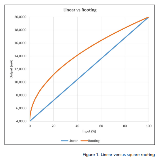
So what to do? To calibrate, you should simply move the first calibration point a bit higher than 0
percent of the input range. If the first calibration point is at 5–10 percent of the input range, you
are already out of the steepest part of the curve, and you can get reasonable readings and error
calculations. Of course, then you do not calibrate the zero point, but your process is normally not
running at zero point either.
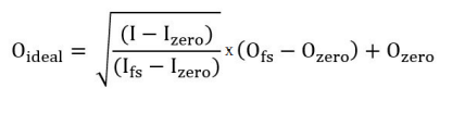
How to calculate the output?
Use the formula below to calculate what the output current should be at a given input point:
Where: